Understanding portfolio performance: contribution and attribution
Suppose a portfolio returned 6.60% last quarter against a benchmark that returned 5.45%, outperforming the benchmark by 115 basis points. The question for the portfolio manager is what drove this outperformance, and whether the calculations reconcile in the next quarter.
1. Contribution and attribution
A portfolio return combines the weights assigned to individual components, such as sectors, with the returns those components earn. Consequently, the total return summarizes the result of the portfolio as a whole. To identify where that return came from, the total can then be separated into the amount generated by each component. This decomposition is called contribution analysis.
For the single period relationships below, assume that no trading takes place during the measurement period and that there are no external cash flows. Let \(i=1,\ldots,n\) identify the portfolio components, let \(w_{P,i}\) denote the beginning weight of component \(i\), and let \(r_{P,i}\) denote its return. The portfolio return \(R_P\) is
The contribution of component \(i\), denoted by \(C_{P,i}\), is the corresponding term in Equation (1.1),
so that the component contributions reconcile with the portfolio return,
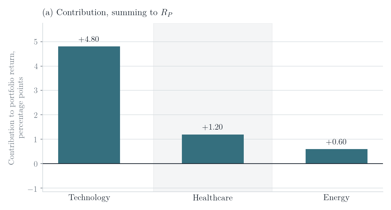
Consider a three sector portfolio with the weights and returns shown in Table 1. Technology contributes \(0.40\times12.0\%=4.80\%\) of the initial portfolio value to the quarter return, Healthcare contributes \(0.30\times4.0\%=1.20\%\), and Energy contributes \(0.30\times2.0\%=0.60\%\). Adding the three contributions gives
| Sector | \(w_{P,i}\) | \(r_{P,i}\) | Calculation | \(C_{P,i}\) |
|---|---|---|---|---|
| Technology | 40% | 12.0% | \(0.40\times12.0\%\) | 4.80% |
| Healthcare | 30% | 4.0% | \(0.30\times4.0\%\) | 1.20% |
| Energy | 30% | 2.0% | \(0.30\times2.0\%\) | 0.60% |
| Total | 100% | 6.60% |
Once performance is evaluated relative to a benchmark, the analysis must also account for the weights and returns of that benchmark. Let \(w_{B,i}\) and \(r_{B,i}\) denote the corresponding benchmark weight and return. The benchmark return \(R_B\) is
For the same three sectors, suppose the benchmark assigns weights of 25%, 35% and 40% to Technology, Healthcare and Energy, with corresponding returns of 10%, 5% and 3%. Equation (1.5) then gives
The difference between the portfolio and benchmark returns, \(R_P-R_B\), is called the arithmetic active return. For the worked example it is
where a positive value indicates that the portfolio outperformed the benchmark, and a negative value indicates that it underperformed. Decomposing the active return is called attribution analysis, where the goal is to identify where performance relative to the benchmark originates. Table 2 sets out what each decomposition requires and what it answers.
| Contribution | Attribution | |
|---|---|---|
| Decomposes | Portfolio return \(R_P\) | Active return \(R_P-R_B\) |
| Benchmark required | No | Yes |
| Inputs | Portfolio weights and returns | Portfolio and benchmark weights and returns |
| Answers | Where did the portfolio return come from? | Where did we gain or lose versus the benchmark? |
2. Combining contributions across periods
A contribution reported in each period is expressed relative to the portfolio value at the start of that period. As the portfolio gains or loses value, that starting value changes. The same reported contribution percentage can therefore represent different amounts of capital in different periods.
Suppose the portfolio starts with a value of 100 and earns 10% during the first period. The portfolio value at the start of the second period is \(100(1+0.10)=110\). If one portfolio segment contributes 3% in each period, the first contribution represents \(100\times0.03=3\) units of value and the second represents \(110\times0.03=3.30\). Directly adding the reported percentages gives \(3\%+3\%=6.00\%\), while the segment has added \(3+3.30=6.30\) units relative to the initial portfolio value of 100. Its contribution over the full measurement period is therefore \(6.30/100=6.30\%\).
The 0.30 percentage point difference between the direct sum and that figure arises because the two contributions are measured from different starting portfolio values.
To express the same issue generally, let \(t=1,\ldots,T\) index the measurement periods. Let \(w_{i,t-1}\) denote the weight of portfolio segment \(i\) at the start of period \(t\), and let \(r_{i,t}\) denote its return during that period. Its contribution is \(C_{i,t}=w_{i,t-1}r_{i,t}\), and the portfolio return during period \(t\) is \(R_{P,t}=\sum_i C_{i,t}\). The compounded portfolio return over the full measurement period is
For two periods, adding the period contributions across all portfolio segments gives \(\sum_i(C_{i,1}+C_{i,2})=R_{P,1}+R_{P,2}\), whereas Equation (2.1) gives
The two expressions differ by the compounding term \(R_{P,1}R_{P,2}\). The task is therefore to construct a contribution for each portfolio segment over the full measurement period that is consistent with the compounded portfolio return. Two methods are used below.
2.1 Method A: Initial weight and compounded segment return
Method A follows the capital allocated to portfolio segment \(i\) at the start of the full measurement period. If the initial portfolio value is \(V_0\), the segment initially holds \(V_0w_{i,0}\). When no trading takes place, that capital remains invested in the segment and compounds at the segment returns,
Equation (2.3) reconciles with the compounded portfolio return in Equation (2.1) when there is no trading, because the capital initially allocated to each portfolio segment then remains invested there throughout the measurement period, so the starting weight and compounded segment return describe the capital that was actually exposed to that segment. Once trading occurs, the amount invested in a portfolio segment can change during the measurement period and its starting weight no longer represents the capital exposed to that segment throughout the period. Method A is then no longer guaranteed to reconcile. Particular trading patterns can still produce exact reconciliation.
2.2 Method B: Period contributions on a common capital base
Method B works directly with the contribution measured in each period. Because \(C_{i,t}\) is measured relative to the portfolio value at the start of period \(t\), contributions from different periods are expressed on different capital bases. Method B makes them comparable by expressing each one relative to the portfolio value at the start of the full measurement period.
By the start of period \(t\), the portfolio has already earned the returns from periods 1 through \(t-1\). Its value relative to the start of the full measurement period has therefore changed by \(\prod_{s=1}^{t-1}(1+R_{P,s})\), which equals one at \(t=1\) because no earlier portfolio returns have been earned. Multiplying the period contribution by that growth factor expresses the contribution relative to the initial capital base,
The earlier numerical example makes each term in Equation (2.4) explicit. The segment contribution is \(C_{i,1}=3\%\) in period 1 and \(C_{i,2}=3\%\) in period 2. For period 1 the growth factor is one, so the adjusted contribution remains 3%. For period 2 the portfolio grew by 10% during period 1, so \(R_{P,1}=10\%\), the growth factor is \(1.10\), and the adjusted contribution is \(3\%\times1.10=3.30\%\). Adding the two adjusted contributions gives \(C_i^{(B)}=3.00\%+3.30\%=6.30\%\), which matches the 6.30% calculated earlier. Since the contributions within each period sum to that period's portfolio return, Method B produces contributions that satisfy
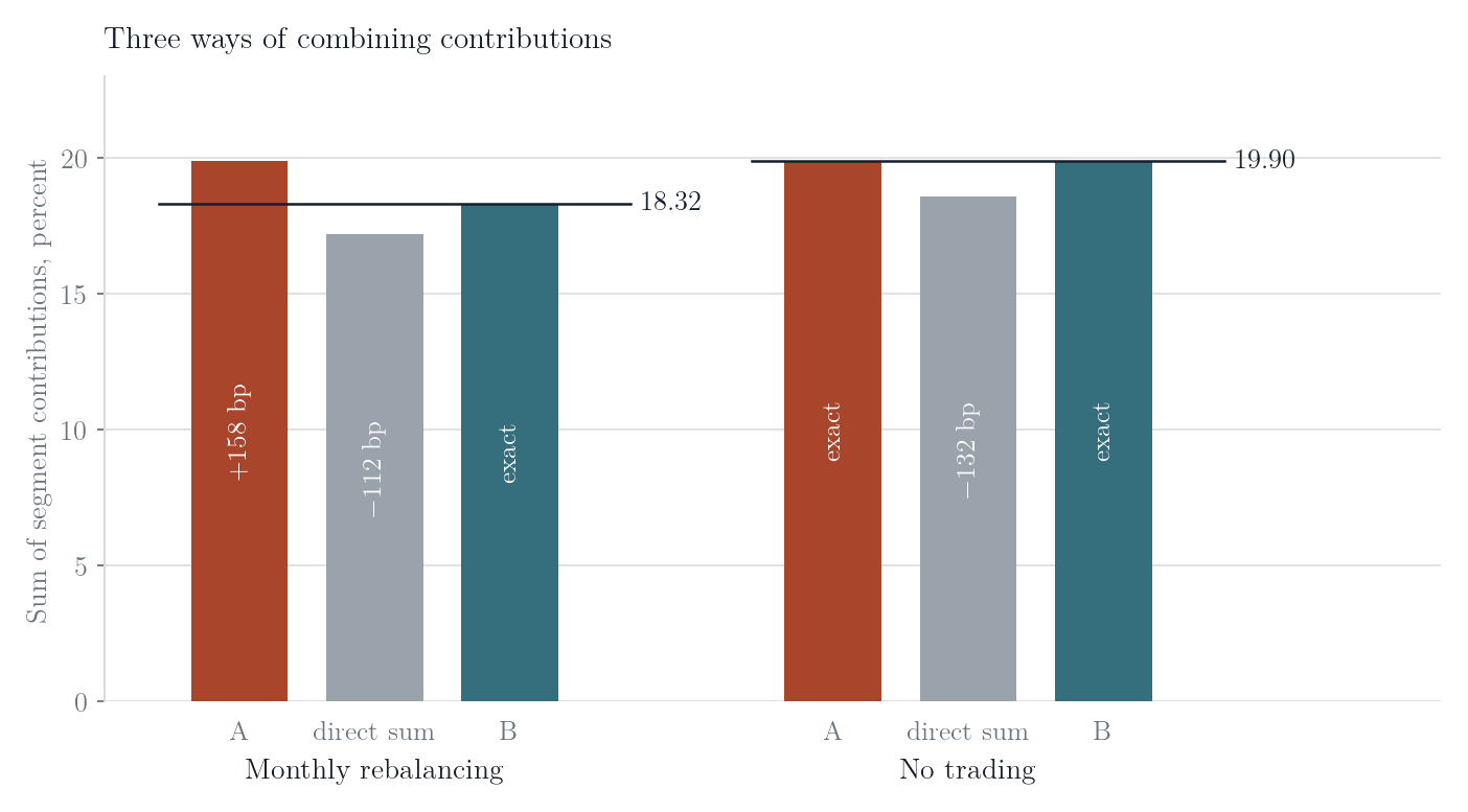
Figure 2 compares Method A, Method B and a direct arithmetic sum of the monthly contributions for a two asset portfolio that starts with 60% in equities and 40% in bonds. Over the twelve month period, equities return 36.9% and bonds return \(-5.6\%\). In the first portfolio path, the weights are reset to 60% and 40% at each month end. Applied to the contributions generated by that path, Method A exceeds the compounded portfolio return by 158 basis points, the direct sum falls short by 112 basis points, and Method B reconciles exactly through Equation (2.5). In the second portfolio path, no trading takes place, so the capital initially allocated to each asset remains invested there throughout the period and Method A also reconciles exactly. The direct sum remains 132 basis points below the compounded portfolio return, because the monthly contributions continue to be measured on changing portfolio values.
3. Single period arithmetic attribution
The arithmetic active return in Equation (1.7) reflects differences between the portfolio and benchmark in both the weights assigned to individual sectors and the returns earned within those sectors. Brinson and Fachler (1985) separate these differences into allocation, selection and interaction effects.
The allocation effect isolates the weight difference by evaluating it against the return of the benchmark sector relative to the benchmark as a whole. For sector \(i\),
Because \(r_{B,i}-R_B\) measures the benchmark sector return relative to the total benchmark return, an overweight produces a positive allocation effect when the sector outperforms the benchmark as a whole, and an underweight produces a positive allocation effect when the sector underperforms the benchmark as a whole.
Once the weight difference has been isolated, performance within the sector can be evaluated at the benchmark weight,
The return difference \(r_{P,i}-r_{B,i}\) compares the return earned by the portfolio holdings within sector \(i\) with the return earned by the corresponding benchmark holdings. Multiplying that return difference by \(w_{B,i}\) measures its contribution to active return at the benchmark sector weight.
The portfolio can differ from the benchmark in both weight and return at the same time. The interaction effect captures the return difference on the portion of the portfolio weight that lies above or below the benchmark weight,
Consider Technology in the worked example. Its portfolio weight is 40%, its benchmark weight is 25%, its portfolio return is 12%, its benchmark return is 10%, and the total benchmark return from Equation (1.6) is 5.45%. Substituting these values into Equations (3.1), (3.2) and (3.3) gives
Technology therefore contributes \(0.6825\%+0.5000\%+0.3000\%=1.4825\%\) to active return. Applying the same calculations to Healthcare and Energy produces Table 3.
| Sector | \(w_P\) | \(r_P\) | \(w_B\) | \(r_B\) | \(A_i\) | \(S_i\) | \(I_i\) | Total |
|---|---|---|---|---|---|---|---|---|
| Technology | 40% | 12.0% | 25% | 10.0% | 0.6825 | 0.5000 | 0.3000 | 1.4825 |
| Healthcare | 30% | 4.0% | 35% | 5.0% | 0.0225 | −0.3500 | 0.0500 | −0.2775 |
| Energy | 30% | 2.0% | 40% | 3.0% | 0.2450 | −0.4000 | 0.1000 | −0.0550 |
| Total | 100% | 6.60% | 100% | 5.45% | 0.9500 | −0.2500 | 0.4500 | 1.1500 |
Across all sectors, the three effects reconcile with the arithmetic active return,
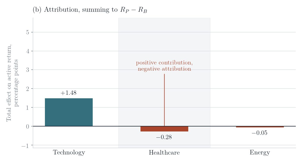
For the worked example, Equation (3.5) becomes \(0.9500\%-0.2500\%+0.4500\%=1.1500\%\), which is the active return calculated in Equation (1.7). Figure 3 reports the total sector effects: Technology contributes 1.4825 percentage points, Healthcare \(-0.2775\) and Energy \(-0.0550\). Healthcare contributes 1.20 percentage points to the portfolio return and has a total attribution effect of \(-0.2775\) percentage points relative to the benchmark.
3.1 Alternative arithmetic attribution conventions
The decomposition above follows Brinson and Fachler (1985), whose allocation effect is given in Equation (3.6).
Brinson, Hood and Beebower (1986) use the allocation effect in Equation (3.7).
The sector allocation effects differ between the two conventions. Their aggregate allocation effects are equal because the portfolio and benchmark weights each sum to one, so \(\sum_i(w_{P,i}-w_{B,i})=0\) and
A separate reporting choice concerns interaction. Combining Equations (3.2) and (3.3) gives
This reporting choice changes how active return is divided between the named effects while preserving the total active return (Ankrim and Hensel, 1994).
4. Linking attribution effects across periods
The compounding problem in Section 2 also appears in attribution, because both the portfolio and benchmark compound through time. Within each period, allocation, selection and interaction reconcile with that period's arithmetic active return through Equation (3.5). Across several periods, adding those arithmetic active returns does not generally reproduce the difference between the separately compounded portfolio and benchmark returns.
For two periods, subtracting the compounded benchmark return from the compounded portfolio return and expanding both products gives
Adding the arithmetic active returns from the two individual periods gives only the first two terms of Equation (4.1), so the arithmetic sum omits the difference between the portfolio and benchmark compounding terms. For example, if the portfolio returns 10% in each period while the benchmark returns 9%, the arithmetic active return is 1 percentage point in each period and the two period sum is 2.00%. The compounded portfolio return is \((1.10)^2-1=21.00\%\) and the compounded benchmark return is \((1.09)^2-1=18.81\%\), so the arithmetic active return over the full measurement period is 2.19%. The 0.19 percentage point gap is the third term of Equation (4.1),
For \(T\) periods, the same issue is that \(\sum_{t=1}^{T}(R_{P,t}-R_{B,t})\) does not generally equal \(R_P^{(1:T)}-R_B^{(1:T)}\). Let \(A_t\), \(S_t\) and \(I_t\) denote the period level allocation, selection and interaction effects after summing the sector effects. Since the single period attribution reconciles, \(A_t+S_t+I_t=R_{P,t}-R_{B,t}\), and adding the attribution effects across periods gives
which does not generally equal the compounded active return. A linking method adjusts the period effects so that the linked allocation, selection and interaction effects reconcile with \(R_P^{(1:T)}-R_B^{(1:T)}\), the difference between the separately compounded portfolio and benchmark returns. Several methods produce exact reconciliation of the aggregate attribution effects, including those of Cariño (1999), Menchero (2000), GRAP (1997), Frongello (2002), and Davies and Laker (2001).
4.1 Linking methods
To use the same notation across the methods, let \(E_t\) denote any one of \(A_t\), \(S_t\) or \(I_t\) in period \(t\). Each method constructs a linked value \(E^{(1:T)}\), and the linked effects are required to satisfy
Cariño (1999) constructs the adjustment from the relationship between arithmetic and logarithmic active returns. For period \(t\), and for the full measurement period, define
Both expressions in Equation (4.5) have a removable singularity when the portfolio and benchmark returns coincide, with limits
The linked effect is then
Menchero (2000) applies a common scale followed by a period specific correction. Let \(a_t=R_{P,t}-R_{B,t}\) denote the arithmetic active return in period \(t\), and define
The scale \(M\) has a removable singularity when the compounded portfolio and benchmark returns coincide, with limit
The residual \(D\) in Equation (4.8) is the amount still required for reconciliation after applying \(M\). The coefficient correction for period \(t\) is proportional to its active return \(a_t\). Since the aggregate attribution effect in period \(t\) equals \(a_t\), the residual adjustment contributed by that period is \(Da_t^{2}\big/\sum_s a_s^{2}\), so the residual is allocated according to squared period active returns. The resulting coefficients are
GRAP (1997) expresses the compounding adjustment directly through the return path. The first product below places the period \(t\) effect on the portfolio value accumulated before the period, and the second carries that effect from period \(t\) to the end of the measurement period using subsequent benchmark returns,
Frongello (2002) reaches the same result recursively. Let \(F_t\) denote the adjusted effect introduced in period \(t\). The current period effect is scaled by portfolio growth accumulated before the period, and the effects accumulated earlier are carried forward at the current benchmark return,
Expanding the recursion in Equation (4.12) produces the multiplier in Equation (4.11), so the recursive and direct constructions produce the same linked effects.
Davies and Laker (2001) construct the full period effects from notional return paths. The allocation notional return combines portfolio weights with benchmark sector returns, and the selection notional return combines benchmark weights with portfolio sector returns,
Compounding the benchmark, allocation notional, selection notional and portfolio paths gives
and the linked effects follow as differences between those compounded paths,
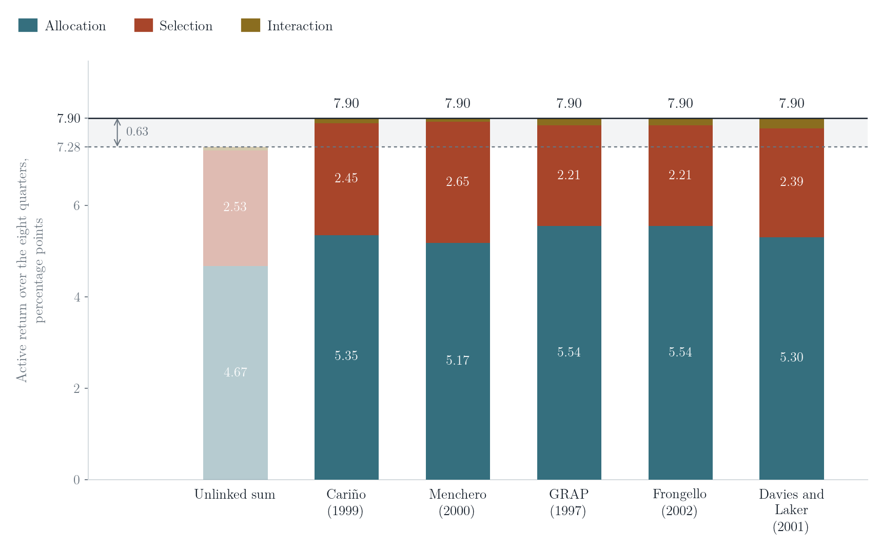
All five methods satisfy Equation (4.4), while the individual allocation, selection and interaction totals can differ because each method distributes the compounding adjustment differently. In the example shown in Figure 4, the unlinked period effects sum to 7.279% and the separately compounded portfolio and benchmark returns produce an active return of 7.9045%, so the required adjustment is \(7.9045\%-7.2790\%=0.6255\%\). Each method closes that gap and reaches the same 7.9045% active return, while the amounts reported as allocation, selection and interaction depend on the chosen linking rule.
5. Data frequency, trading, drift and costs
The attribution equations treat portfolio weights as inputs. In practice, those weights can change because one component appreciates relative to the rest of the portfolio, because securities are bought or sold, or because cash flows change the quantities held. A weight observed at one point in time shows the exposure held at that date without revealing the path by which the portfolio reached it.
To see how that path can change without any trading, consider the effect of returns alone. If there is no trading and no external cash flow, the capital invested in segment \(i\) grows from \(w_{i,t-1}\) to \(w_{i,t-1}(1+r_{i,t})\), while the portfolio as a whole grows from one unit of capital to \(1+R_{P,t}\). The end of period weight produced by returns alone is therefore
If \(r_{i,t}\) exceeds \(R_{P,t}\), then Equation (5.1) implies that \(w_{i,t}^{\mathrm{drift}}\) exceeds \(w_{i,t-1}\), so the segment becomes a larger share of the portfolio even though no trade has taken place. If \(r_{i,t}\) falls below \(R_{P,t}\), its weight falls. Relative performance alone can therefore change the portfolio weight.
The same observed weight can be reached through different histories. Figure 5 shows three portfolio paths that all finish with a weight of 55% against a benchmark weight of 50%. In the first path, the portfolio holds 55% throughout the four quarters. In the second, it starts at 50% and is increased to 55% through trading. In the third, it starts at 50% and reaches 55% through relative price movements without a trade. All three finish with the same 5 percentage point active weight, which identifies the exposure at the end of quarter 4 without identifying whether the overweight was maintained, traded into, or reached through drift.
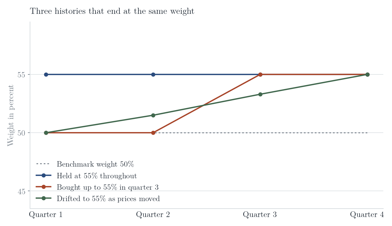
Distinguishing among those paths requires observations before the endpoint. The frequency of the holdings data therefore determines how closely the attribution can follow changes in the portfolio through time. Suppose a portfolio segment has a weight of 50% at the start of a month and is increased to 60% halfway through the month. If the month is treated as one attribution period using only the opening holdings, the calculation uses the 50% weight even though the portfolio holds 60% during the second half of the month. Weekly or daily holdings allow the attribution period to be shortened and the weight to be updated closer to the time at which the portfolio changes. Holdings based attribution is commonly calculated from monthly, weekly or daily position data (Bacon, 2019).
More frequent holdings observations provide a more detailed record of the portfolio through time. Each observation still captures the positions held at a particular point. When a position changes between two consecutive observations, the holdings data identify the resulting change without revealing the sequence, timing or execution prices of the transactions that produced it. Transaction data provide this additional information and become increasingly important as turnover rises, because a greater share of the portfolio's exposure can change between successive holdings observations.
5.1 Transaction costs
Transaction data also make it possible to separate recorded trading costs from the investment effects. Let \(R_{P,t}^{\mathrm{gross}}\) denote the portfolio return before those costs and \(R_{P,t}^{\mathrm{net}}\) the return after them, and define the transaction cost effect as
where \(C_t^{\mathrm{cost}}<0\) whenever recorded transaction costs are positive. When allocation, selection and interaction are calculated from gross returns, they reconcile with the gross active return,
Adding Equation (5.2) to Equation (5.3) gives the reconciliation with the net active return,
The transaction cost effect therefore shows how much recorded trading costs reduced active return. If individual transactions are classified by their purpose, the same costs can also be assigned to the trading activity that generated them.
6. Extensions beyond standard sector attribution
The attribution model developed above uses portfolio and benchmark weights together with sector returns. Other sources of active return require additional information, because bond returns depend on interest rate exposure, international returns depend on currency exposure, and factor models relate returns to systematic sources of risk.
6.1 Fixed income attribution
Bond prices respond to changes in yields, and the size of that response depends on modified duration. Let \(P\) denote the bond price, \(D_{\mathrm{mod}}\) its modified duration and \(\Delta y\) the change in yield. For a small yield change,
A portfolio can therefore earn active return from a different interest rate exposure even when its market weights are similar to those of the benchmark. The weighted duration approach separates differences in total duration from the distribution of duration across markets and from the yield changes experienced within those markets (Van Breukelen, 2000).
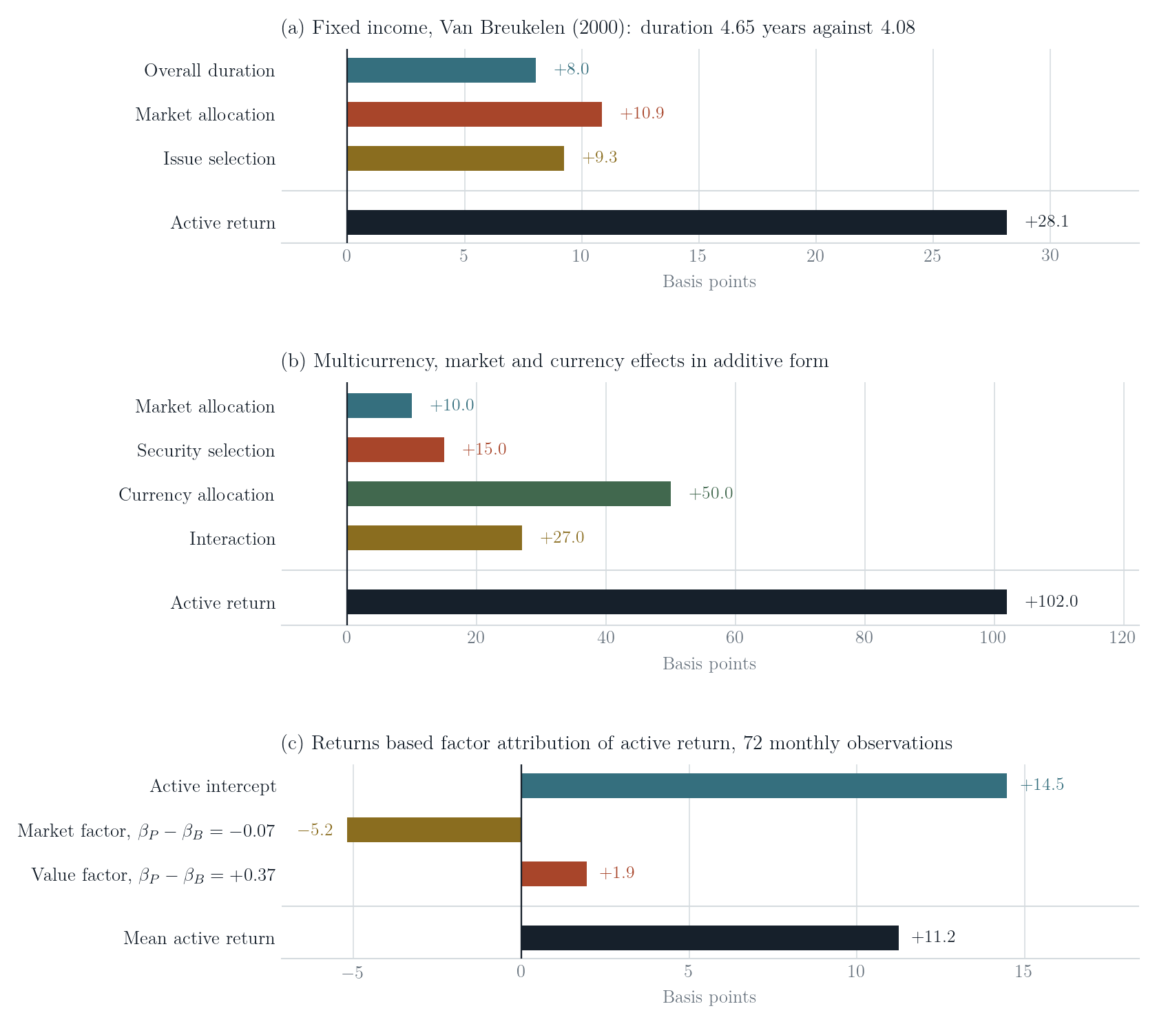
Panel (a) of Figure 6 uses Government and Credit bonds. The portfolio has a modified duration of 4.65 years compared with 4.08 years for the benchmark. The benchmark duration weighted yield change is negative, so the portfolio benefits from carrying an additional 0.57 years of duration and produces an overall duration effect of 8.05 basis points. The portfolio also places a larger share of its duration in Government bonds, where benchmark yields fall, and a smaller share in Credit, where benchmark yields rise, producing a market allocation effect of 10.85 basis points. Within Government bonds, portfolio yields fall more than benchmark yields, while the opposite occurs within Credit, and the larger Government advantage leaves a positive issue selection effect of 9.25 basis points. In this duration based illustration, the three effects sum to \(8.05+10.85+9.25=28.15\) basis points.
6.2 Multicurrency attribution
A foreign investment produces both a local market return and a currency return. Let \(R_{\mathrm{local}}\) denote the local return and \(R_{\mathrm{FX}}\) the return from the exchange rate. In simple returns,
Currency positions can also differ from the exposures implied by the underlying securities, because they can be altered using forward contracts. Multicurrency attribution therefore separates market and currency performance (Ankrim and Hensel, 1994; Karnosky and Singer, 1994). Panel (b) of Figure 6 uses an additive approximation that drops the cross term in Equation (6.2),
Karnosky and Singer (1994) formulate their attribution framework using continuously compounded returns and local return premiums, with local cash returns incorporated into the currency component through interest rate parity.
Panel (b) allocates 60% of the portfolio to the United States compared with 50% in the benchmark, and 40% to Japan compared with 50% in the benchmark. The United States has the higher local benchmark return, so the relative weights produce a positive market allocation effect of 10 basis points. The currency return is 3% for the United States and \(-2\%\) for Japan, so the same weight differences produce a 50 basis point currency allocation effect. Security selection contributes 15 basis points, because the portfolio outperforms within the United States and underperforms within Japan, with the United States advantage larger at the benchmark weights. Interaction contributes another 27 basis points, because the portfolio places more weight in the market where its local portfolio return exceeds its local benchmark return. Under the additive approximation in Equation (6.3), the four effects reconcile as \(10+15+50+27=102\) basis points.
6.3 Factor based attribution
Factor based attribution relates active return to differences between portfolio and benchmark exposures to systematic return sources. Returns based analysis estimates those exposures from a time series of portfolio returns and factor returns (Sharpe, 1992). For the portfolio relative to its benchmark, let \(F_t\) contain the factor returns in period \(t\), and let \(\beta_P\) and \(\beta_B\) denote the corresponding portfolio and benchmark exposures. The active return can then be represented as
where \(\alpha\) is the active intercept and \(\varepsilon_t\) is the part of active return not fitted by the included factors. Panel (c) of Figure 6 estimates Equation (6.4) from 72 monthly observations using market and value factors. The portfolio market exposure is 0.07 below the benchmark exposure, and the positive average market factor return reduces mean active return by 5.2 basis points. The portfolio value exposure is 0.37 above the benchmark exposure, and the positive average value factor return adds 1.9 basis points. The estimated active intercept is 14.5 basis points. Because the ordinary least squares regression includes an intercept, the sample mean of the residual is zero, so the reported mean contributions reconcile with mean active return, \(14.5-5.2+1.9=11.2\) basis points per month.
7. Conclusion
Key Takeaways
- Contribution decomposes the portfolio return \(R_P\). Attribution decomposes the active return \(R_P-R_B\). A portfolio segment can contribute positively to the portfolio return and have a negative attribution effect relative to the benchmark.
- Across several periods, contribution calculations must account for compounding. Method B does so by expressing period contributions on a common initial capital base. Arithmetic attribution effects require a linking method before they can be combined across periods and reconciled with compounded active return.
- Allocation, selection and interaction describe realized return differences. Their values do not by themselves identify how a position arose, adjust for differences in risk, or establish repeatable investment skill.
- The attribution model must represent the sources of return relevant to the portfolio. Fixed income attribution incorporates interest rate exposure, multicurrency attribution separates market and currency effects, and factor attribution measures active systematic exposures.
- Reported attribution results depend on the benchmark and on choices such as the allocation convention, the treatment of interaction, the linking method, the data frequency and the treatment of transaction costs. These choices should be stated, and the reported effects should reconcile with the corresponding portfolio and benchmark returns.
References
Ankrim, E. M., and Hensel, C. R. (1994). Multicurrency performance attribution. Financial Analysts Journal 50(2), 29–35.
Bacon, C. R. (2019). Performance Attribution: History and Progress. CFA Institute Research Foundation.
Brinson, G. P., and Fachler, N. (1985). Measuring non-U.S. equity portfolio performance. Journal of Portfolio Management 11(3), 73–76.
Brinson, G. P., Hood, L. R., and Beebower, G. L. (1986). Determinants of portfolio performance. Financial Analysts Journal 42(4), 39–44.
Cariño, D. R. (1999). Combining attribution effects over time. Journal of Performance Measurement 3(4), 5–14.
Davies, O., and Laker, D. (2001). Multiple-period performance attribution using the Brinson model. Journal of Performance Measurement 6(1), 12–22.
Frongello, A. S. B. (2002). Attribution linking: proofed and clarified. Journal of Performance Measurement 7(1), 54–67.
GRAP, Groupe de Recherche en Attribution de Performance (1997). Synthèse des modèles d'attribution de performance. Paris.
Karnosky, D. S., and Singer, B. D. (1994). Global Asset Management and Performance Attribution. Research Foundation of the Institute of Chartered Financial Analysts, Charlottesville, VA.
Menchero, J. G. (2000). An optimized approach to linking attribution effects over time. Journal of Performance Measurement 5(1), 36–42.
Sharpe, W. F. (1992). Asset allocation: management style and performance measurement. Journal of Portfolio Management 18(2), 7–19.
Van Breukelen, G. (2000). Fixed income attribution. Journal of Performance Measurement 4(4), 61–68.