Portfolio Evaluation and Return Analysis
Portfolio evaluation lies at the heart of successful investing, whether you manage your own money or oversee larger institutional portfolios. At its core, a portfolio is simply the allocation of capital across a variety of assets, and one of the most crucial questions any investor must ask is how to measure whether that allocation is truly working. The challenge does not end with selecting certain stocks, bonds, or cryptocurrencies; equally important is understanding how returns are calculated, how risk is managed, and how to adjust or rebalance your positions over time. In the absence of a solid framework, an investor might rely on guesswork, simplistic heuristics, or emotional impulses. By contrast, a well-grounded approach to portfolio evaluation provides a systematic, evidence-based way to diagnose performance and decide how to pivot in response to shifting market conditions.
A fundamental aspect of any portfolio discussion revolves around how price data are modeled. Suppose we track a universe of \(N\) assets at each time step \(t\). We denote their prices by a vector \[\mathbf{p}_t \;=\; \bigl(p_{1,t},\, p_{2,t},\, \dots,\, p_{N,t}\bigr)^\top,\] where \(p_{i,t}\) is the price of asset \(i\) at time \(t\). A common step in portfolio analysis is to convert these raw prices into returns. Two widely used definitions appear in practice: linear and logarithmic returns. The linear return for asset \(i\) between periods \(t-1\) and \(t\) is given by \[r_{i,t}^{\mathrm{lin}} \;=\; \frac{p_{i,t} \;-\; p_{i,t-1}}{p_{i,t-1}},\] meaning that if \(p_{i,t-1} = 100\) and \(p_{i,t} = 105\), then \(r_{i,t}^{\mathrm{lin}} = 0.05\) (i.e., a 5% gain). By contrast, the logarithmic return is \[r_{i,t}^{\mathrm{log}} \;=\; \ln\bigl(p_{i,t}\bigr)\;-\;\ln\bigl(p_{i,t-1}\bigr),\] so if \(p_{i,t-1} = 100\) and \(p_{i,t} = 105\), then \(r_{i,t}^{\mathrm{log}} = \ln(105) - \ln(100)\approx 0.0488\). Because \(\ln(105/100)\) is slightly less than 0.05, the log-return is smaller but still close to the linear return when changes are modest.
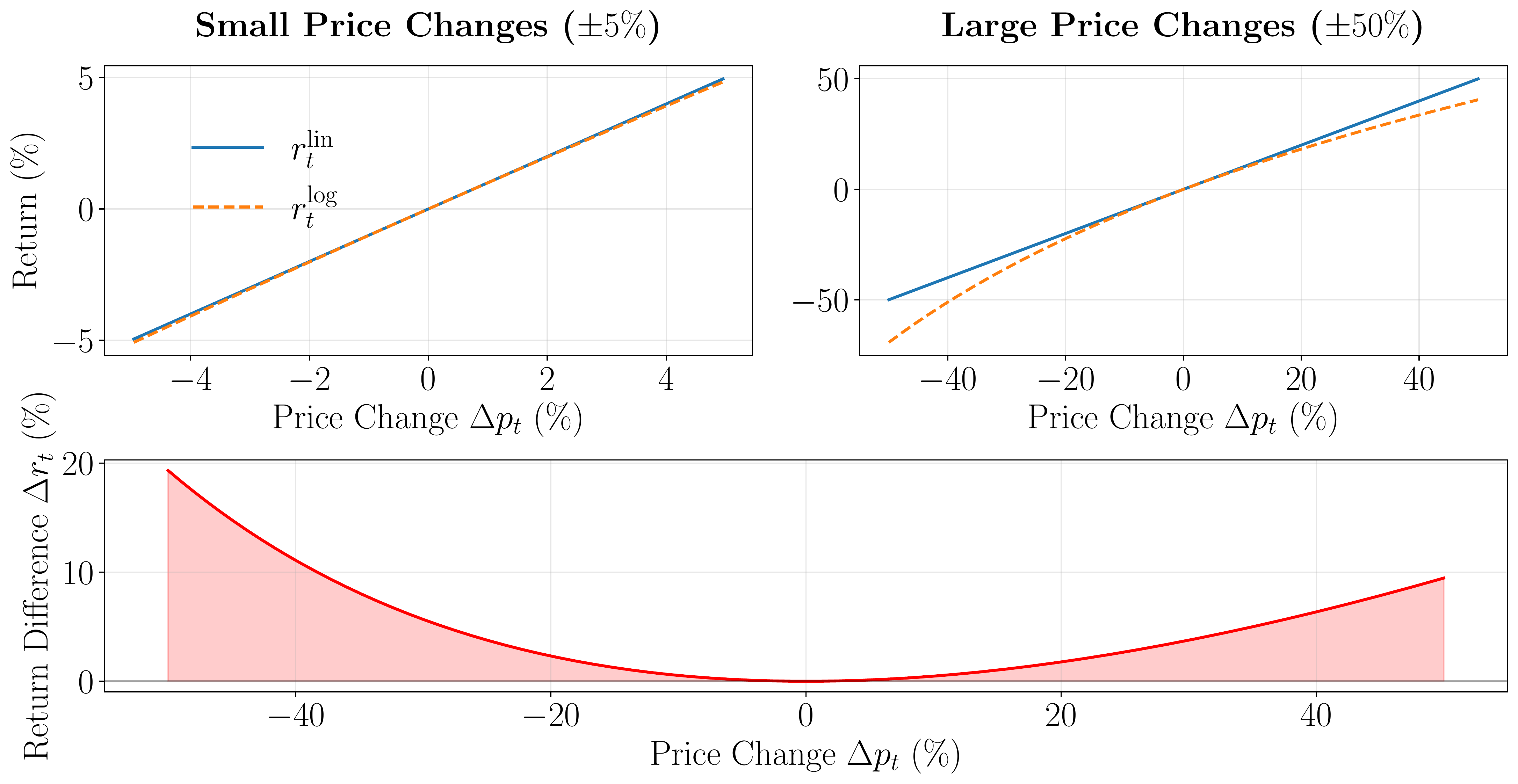
Figure 1 demonstrates how linear and log-returns behave under varying magnitudes of price changes. In the top-left panel, where the price change is limited to \(\pm 5\%\), the two measures are nearly indistinguishable. This visually reinforces the commonly stated rule of thumb that, for small movements, \[r_{i,t}^{\mathrm{lin}} \;\approx\; r_{i,t}^{\mathrm{log}}.\] However, the top-right panel, which extends the range to \(\pm 50\%\), shows a more noticeable gap. As an example, a 50% price decline translates to \(-50\%\) in linear terms but becomes \(\ln(0.5)\approx -69.3\%\) in log terms. To quantify the mismatch, the bottom plot measures \[\Delta r_t \;=\; \bigl(r_{t}^{\mathrm{lin}} - r_{t}^{\mathrm{log}}\bigr),\] revealing that \(\Delta r_t\approx 0\) for small fluctuations but widens significantly for larger positive or negative moves.
In an environment where price moves are small and frequent—for instance, intraday trading on highly liquid stocks—this difference is minor. However, once swings become larger, the two forms of returns begin to yield distinctly different perspectives on profit, risk, and even performance metrics such as volatility.
Another important concept behind logarithmic returns is their time additivity. If we denote daily log-returns by \(r_{1}^{\mathrm{log}}, r_{2}^{\mathrm{log}},\dots,r_{T}^{\mathrm{log}}\), the total log-return over \(T\) periods is \[\sum_{t=1}^T r_{t}^{\mathrm{log}},\] making it straightforward to shift between daily, weekly, or monthly time scales by simple addition. By contrast, linear returns must be multiplied (rather than summed) to capture long-horizon effects. For example, two consecutive daily returns of \(+1\%\) and \(+2\%\) yield a combined gain of \((1+0.01)\times(1+0.02) -1=3.02\%\), not simply \(3\%\). This additive property is a key reason why log-returns are favored in many statistical models and volatility estimations, even though investors ultimately book profits and losses in linear space.
Because real-world profit-and-loss statements remain anchored to linear percentages, traders and portfolio managers must be mindful of these two perspectives. A \(-50\%\) linear drop literally halves one's capital, whereas a log-return of \(-0.5\) corresponds to a more modest \(\exp(-0.5)\approx-39\%\) in linear terms. This discrepancy has immediate consequences for risk metrics such as drawdowns. A drawdown tracks how far the portfolio's value has fallen from its historical peak—literally, "how many dollars are missing". Even if a model indicates a log-return of \(-0.5\), the actual portfolio value might be down by 50% when you check your account balance, underscoring the practical difference.
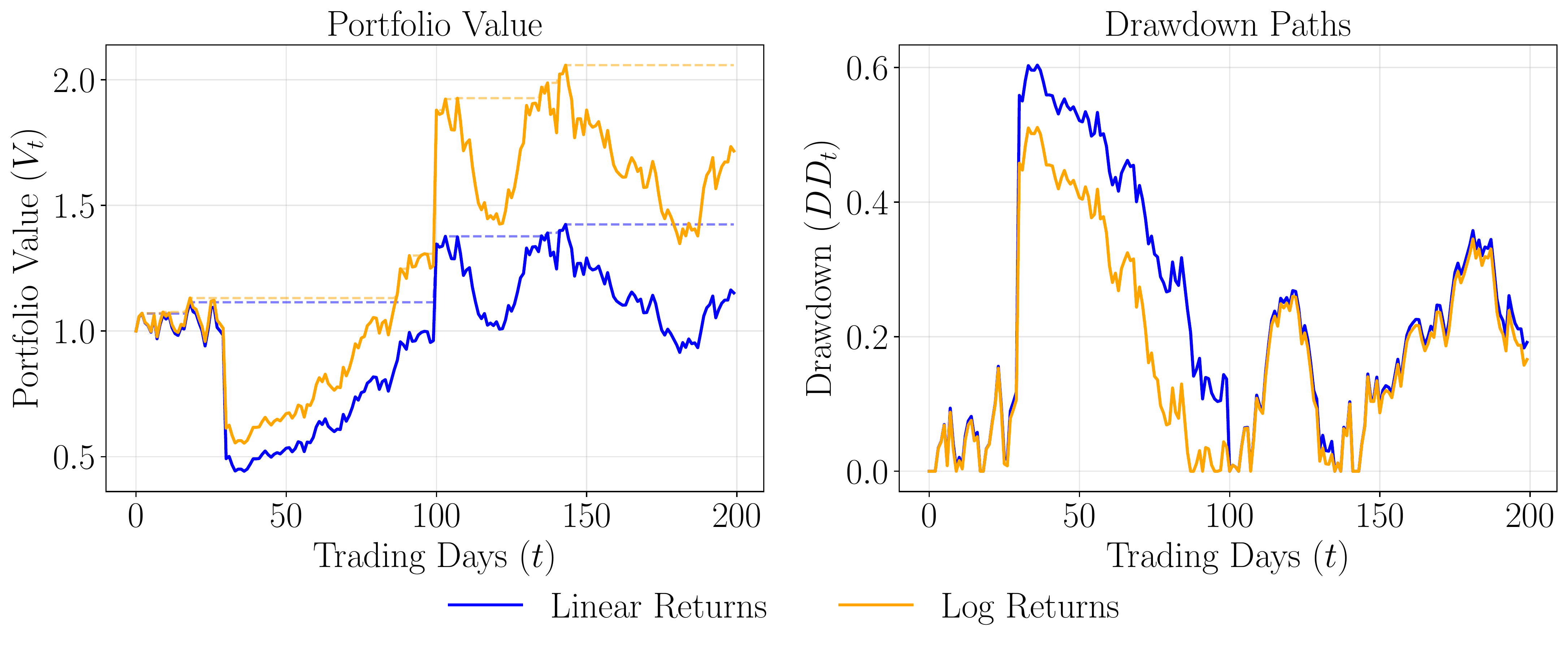
Figure 2 shows an example simulation in which the same sequence of daily shocks is applied to a hypothetical portfolio under two interpretations: one treats each shock as a linear return, while the other treats it as a log-return. We insert two major events—a \(-50\%\) crash on day 30 and a \(+40\%\) surge on day 100—to highlight where the two compounding regimes diverge. In the left panel, we track the portfolio's net asset value \(V_t\) over time, along with its running maximum, \(\max_{\tau \le t} V_\tau\). Under the linear scenario, a \(-50\%\) daily return literally halves the portfolio on day 30, whereas the log-based approach for a shock of \(-0.5\) results in a multiplier of \(\exp(-0.5)\approx 0.6065\), corresponding to a less dire \(-39.35\%\) drop in linear terms.
The right panel in Figure 2 plots the drawdown, \[\mathrm{DD}_t \;=\; 1 \;-\; \frac{V_t}{\max_{\tau \le t} \, V_\tau},\] revealing how much each approach falls beneath its previous peak. Because the linear path suffers the full brunt of \(-50\%\), it hits a deeper trough and takes longer to recover, especially if subsequent rebounds are modest. By contrast, the log-based path experiences a smaller "percentage drop", which may facilitate a quicker rebound in modeling terms. Still, from a purely numerical standpoint, an account balance sliced in half is impossible to ignore, and that is precisely why actual P&L calculations stick to linear returns.
In practice, a robust portfolio evaluation thus blends these two views: log-returns for certain statistical or econometric tasks (where time-additivity and multiplicative processes reign), and linear returns for real-world profit, loss, drawdown, and risk-limits reporting. Smaller, low-volatility markets can mask the difference between them, but in the presence of large negative shocks (e.g., market crashes) or dramatic positive runs (e.g., bubble-like surges), the gap becomes stark. Deciding which measure to employ should therefore depend on both the magnitude of the price changes you expect and the type of risk or performance metric you aim to analyze.